机器学习可以从数据中得到有用的见解. 目标是纵观Spark MLlib,采取适合的算法从数据集中生偏见解。对 Twitter的数据集, 采取非监督集群算法来辨别与Apache
Spark相干的tweets . 初始输入是混合在1起的tweets。 首先提取相干特性, 然后在数据集中使用机器学习算法 , 最后评估结果和性能.
本章重点以下:
•了解 Spark MLlib 模块及其算法,还有典型的机器学习流程 .
• 预处理 所收集的Twitter 数据集提取相干特性, 利用非监督集群算法辨认Apache Spark-
相干的tweets. 然后, 评估得到的模型和结果.
• 描写Spark 机器学习的流水线
Spark MLlib 在利用架构中的位置
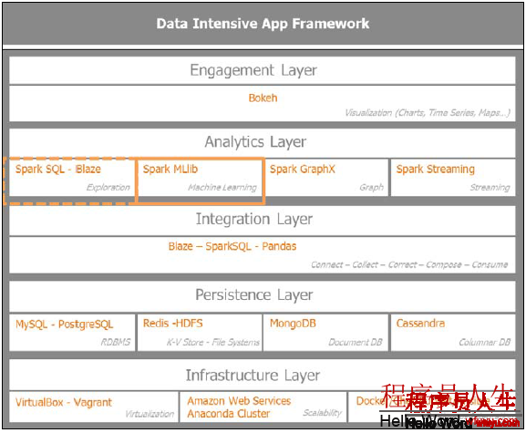
先看1下数据学习在数据密集型利用架构中的位置,集中关注分析层,准确1点说是机器学习。这是批处理和流处理数据学习的基础,它们只是推测的规则不同。
下图指出了重点, 分析层处理的探索式数据分析工具 Spark SQL和Pandas外 还有机器学习模块.
Spark MLlib 算法分类
Spark MLlib 是1个更新很快的模块,新的算法不断地引入到 Spark中.
下图提供了 Spark MLlib 算法的高层通览,并根据传统机器学习技术的体系或数据的连续性进行了分组:
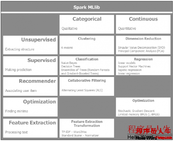
根据数据的类型,将 Spark MLlib 算法分成两栏, 性质无序或数量连续的 . 我们将数据辨别为无序的性质数据和数量连续的数据。1个性质数据的例子:在给定大气压,温度,云的类型和显现, 天气是晴朗,干燥,多雨,或阴天时
时,预测她是不是穿着男性上装,这是离散的值。 另外一方面, 给定了位置,住房面积,房间数,想预测房屋的价格 , 房地产可以通过线性回归预测。
本例中,讨论数量连续的数据。
水平分组反应了所使用的机器学习算法的类型。监督和非监督机器学习取决于训练的数据是不是标注。非监督学习的挑战是对非标注数据使用学习算法。目标是发现输入中隐含的结构。
而监督式学习的数据是标注过的。 重点是对连续数据的回归预测和离散数据的分类.
机器学习的1个重要门类是推荐系统,主要是利用了协同过滤技术。 Amazon 和 Netflix 有自己非常强大的 推荐系统.
随机梯度降落是合适于Spark散布计算的机器学习优化技术之1。对处理大量的文本,Spark提供了特性提取和转换的重要的库例如: TF-IDF , Word2Vec, standard scaler, 和normalizer.
监督和非监督式学习
深入研究1下Spark MLlib 提供的传统的机器学习算法 . 监督和非监督机器学习取决于训练的数据是不是标注. 区分无序和连续取决于数据的离散或连续.
下图解释了 Spark MLlib 监督和非监督时算法及预处理技术 :
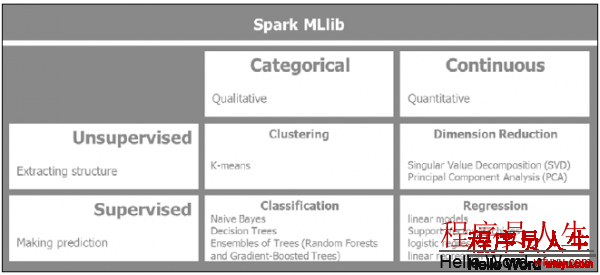
下面时Spakr MLlib中的监督和非监督算法和与预处理技术:
• Clustering 聚类: 1个非监督式机器学习技术,数据是没有标注的,目的是数据中提取结构:
∞ K-Means: 从 K个不同聚类中进行数据分片
∞ Gaussian Mixture: 基于组件的最大化后验几率聚类
∞ Power Iteration Clustering(PIC): 根据图顶点的两两边的类似程度聚类
∞ Latent Dirichlet Allocation (LDA): 用于将文本文档聚类成话题
∞ Streaming K-Means: 使用窗口函数将进入的数据活动态的进行K-Means聚类
• Dimensionality Reduction: 目的在减少特性的数量. 基本上, 用于削减数据噪音并关注关键特性:
∞ Singular Value Decomposition (SVD): 将矩阵中的数据分割成简单的成心义的小片,把初始矩阵生成3个矩阵.
∞ Principal Component Analysis (PCA): 以子空间的低维数据逼近高维数据集..
• Regression and Classification: 当分类器将结果分成类时,回归使用标注过的训练数据来预测输出结果。分类的变量是离散无序的,回归的变量是连续而有序的
:
∞
Linear Regression Models (linear regression, logistic regression,
and support vector machines): 线性回归算法可以表达为凸优化问题,目的是基于有权重变量的向量使目标函数最小化. 目标函数通过函数的
正则部份控制函数的复杂性,通过函数的损失部份控制函数的误差.
∞
Naive Bayes: 基于给定标签的条件几率来预测,基本假定是变量的相互独立性。
∞
Decision Trees: 它履行了特性空间的递归2元划分,为了最好的划分分割需要将树状节点的信息增益最大化。
∞
Ensembles of trees (
Random Forests and Gradient-
Boosted Trees):
树集成算法结合了多种决策树模型来构建1个高性能的模型,它们对分类和回归是非常直观和成功的。
• Isotonic Regression保序回归: 最小化所给数据和可观测响应的均方根误差.
其他学习算法
Spark MLlib 还提供了很多其它的算法,广泛地说有3种其它的机器学习算法:
推荐系统, 优化算法, 和特点提取.
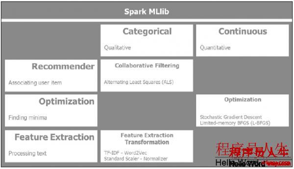
下面当前是 MLlib 中的其它算法:
• Collaborative filtering: 是推荐系统的基础,创建用户-物品关联矩阵,目标是填充差异。基于其它用户与物品的关联评分,为没有评分的目标用户推荐物品。在散布式计算中, ALS (Alternating Least Square)是最成功的算法之1:
∞ Alternating Least Squares交替最小2乘法: 矩阵分解技术采取了隐性反馈,时间效应和置信水平,把大范围的用户物品矩阵分解成低维的用户物品因子,通过替换因子最小化2次损失函数。
• Feature extraction and transformation: 这些是大范围文档处理的基础,包括以下技术:
∞ Term Frequency: 搜素引擎使用Search engines use TF-IDF 对语料库中的文档进行等级评分。机器学习中用它来判断1个词在文档或语料库中的重要性. 词频统计所肯定的权重取决于它在语料库中出现的频率。 词频本身可能存在毛病导向比如过分强调了类似 the, of, or and 等这样无意义的信息辞汇. 逆文档频率提供了特异性或信息量的度量,辞汇在语料库中所有文档是不是常见。
∞ Word2Vec: 包括了两个模型 Skip-Gram 和Continuous
Bag of Word. Skip-Gram 预测了1个给定辞汇的邻近词, 基于辞汇的滑动窗口; Continuous Bag of
Words 预测了所给定邻近辞汇确当前词是甚么.
∞ Standard Scaler: 作为预处理的1部份,数据集常常通过平均去除和方差缩放来标准化. 我们在训练数据上计算平均和标准偏差,并利用一样的变形来测试数据.
∞ Normalizer: 在缩放样本时需要规范化. 对点积或核心方法这样的2次型非常有用。
∞ Feature selection: 通过选择模型中最相干的特点来下降向量空间的维度。
∞ Chi-Square Selector: 1个统计方法来丈量两个事件的独立性。
• Optimization: 这些 Spark MLlib 优化算法聚焦在各种梯度降落的技术。 Spark 在散布式集群上提供了非常有效的梯度降落的实现,通过本地极小的迭代完成梯度的快速降落。迭代所有的数据变量是计算密集型的:
∞ Stochastic Gradient Descent: 最小化目标函数即
微分函数的和. 随机梯度降落仅使用了1个训练数据的抽样来更新1个特殊迭代的参数,用来解决大范围稀疏机器学习问题例如文本分类.
• Limited-memory BFGS (L-BFGS): 文如其名,L-BFGS使用了有限内存,合适于Spark MLlib 实现的散布式优化算法。
Spark MLlib data types
MLlib 支持4种数据类型: local vector, labeled point, local matrix,
and distributed matrix. Spark MLlib 算法广泛地使用了这些数据类型:
• Local vector: 位于单机,可以是紧密或稀疏的:
∞ Dense vector 是传统的 doubles 数组. 例如[5.0, 0.0, 1.0, 7.0].
∞ Sparse vector 使用整数和double值. 稀疏向量 [5.0, 0.0, 1.0, 7.0] 应当是 (4,
[0, 2, 3], [5.0, 1.0, 7.0]),表明了向量的维数.
这是 PySpark中1个使用本地向量的例子:
import numpy as np
import scipy.sparse as sps
from pyspark.mllib.linalg import Vectors # NumPy array for dense vector. dvect1 = np.array([5.0, 0.0, 1.0, 7.0]) # Python list for dense vector. dvect2 = [5.0, 0.0, 1.0, 7.0] # SparseVector creation svect1 = Vectors.sparse(4, [0, 2, 3], [5.0, 1.0, 7.0]) # Sparse vector using a single-column SciPy csc_matrix svect2 = sps.csc_matrix((np.array([5.0, 1.0, 7.0]), np.array([0, 2, 3])), shape = (4, 1))
• Labeled point. 1个标注点是监督式学习中的1个有标签的紧密或稀疏向量. 在2元标签中, 0.0 代表负值, 1.0 代表正值.
这有1个PySpark中标注点的例子:
from pyspark.mllib.linalg import SparseVector
from pyspark.mllib.regression import LabeledPoint
# Labeled point with a positive label and a dense feature vector.
lp_pos = LabeledPoint(1.0, [5.0, 0.0, 1.0, 7.0])
# Labeled point with a negative label and a sparse feature vector.
lp_neg = LabeledPoint(0.0, SparseVector(4, [0, 2, 3], [5.0, 1.0, 7.0]))
• Local Matrix: 本地矩阵位于单机上,具有整型索引和double的值.
这是1个 PySpark中本地矩阵的例子:
from pyspark.mllib.linalg import Matrix, Matrices # Dense matrix ((1.0, 2.0, 3.0), (4.0, 5.0, 6.0)) dMatrix = Matrices.dense(2, 3, [1, 2, 3, 4, 5, 6]) # Sparse matrix ((9.0, 0.0), (0.0, 8.0), (0.0, 6.0)) sMatrix = Matrices.sparse(3, 2, [0, 1, 3], [0, 2, 1], [9, 6, 8])
• Distributed Matrix: 充分利用 RDD的成熟性,散布式矩阵可以在集群中同享
. 有4种散布式矩阵类型: RowMatrix, IndexedRowMatrix,
CoordinateMatrix, 和 BlockMatrix:
∞ RowMatrix: 使用多个向量的1个 RDD,创建无意义索引的行散布式矩阵叫做 RowMatrix.
∞ IndexedRowMatrix: 行索引是成心义的. 首先使用IndexedRow 类创建1个 带索引行的RDDFirst,
再创建1个 IndexedRowMatrix.
∞ CoordinateMatrix: 对表达巨大而稀疏的矩阵非常有用。CoordinateMatrix 从MatrixEntry的RDD创建,用类型元组 (long, long, or float)来表示。
∞ BlockMatrix: 从 子矩阵块的RDDs创建,
子矩阵块形如 ((blockRowIndex, blockColIndex),
sub-matrix).
机器学习的工作流和数据流
除算法, 机器学习还需要处理进程,我们将讨论监督和非监督学习的典型流程和数据流.
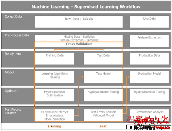
监督式学习工作流程
在监督式学习中, 输入的训练数据集是标注过的. 1个重要的话数据实践是分割输入来训练和测试, 和严重相应的模式.完成监督式学习有6个步骤:
• Collect the data: 这个步骤依赖于前面的章节,保证数据正确的容量和颗粒度,使机器学习算法能够提供可靠的答案.
• Preprocess the data: 通过抽样检查数据质量,添补遗漏的数据值,缩放和规范化数据。同时,定义特点提取处理。典型地,在大文本数据集中,分词,移除停词,词干提取 和 TF-IDF. 在监督式学习中,分别将数据放入训练和测试集。我门也实现了抽样的各种策略, 为交叉检验分割数据集。
• Ready the data: 准备格式化的数据和算法所需的数据类型。在 Spark MLlib中, 包括 local vector, dense 或 sparse vectors, labeled points, local matrix, distributed matrix with row matrix, indexed row matrix, coordinate matrix, 和 block matrix.
• Model: 针对问题使用算法和取得最合适算法的评估结果,可能有多种算法合适同1问题; 它们的性能存储在评估步骤中以便选择性能最好的1个。 我门可以实现1个综合方案或模型组合来得到最好的结果。
• Optimize: 为了1些算法的参数优化,需要运行网格搜索。这些9参数取决于训练,测试和产品调优的阶段。
• Evaluate: 终究给模型打分,并综合准确率,性能,可靠性,伸缩性 选择最好的1个模型。 用性能最好的模型来测试数据来探明模型预测的准确性。1旦对调优模型满意,就能够到生产环境处理真实的数据了 .
监督式机器学习的工作流程和数据流以下图所示:
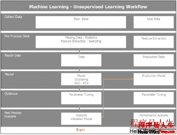
非监督式学习工作流程
与监督式学习相对,非监督式学习的初始数据使没有标注的,这是真实生活的情形。通过聚类或降维算法提取数据中的结构, 在非监督式学习中,不用分割数据到训练和测试中,由于数据没有标注,我们不能做任何预测。训练数据的6个步骤与监督式学习中的那些步骤类似。1旦模型训练过了,将评估结果和调优模型,然后发布到生产环境。
非监督式学习是监督式学习的初始步骤。 也即是说, 数据降维先于进入学习阶段。
非监督式机器学习的工作流程和数据流表达以下:
感受1下从Twitter提取到的数据,理解数据结构,然后运行 K-Means 聚类算法 . 使用非监督式的处理和数据流程,步骤以下:
1. 组合所有的 tweet文件成1个 dataframe.
2.
解析 tweets, 移除停词,提取表情符号,提取URL, 并终究规范化词 (如,转化为小写,移除标点符号和数字).
3. 特点提取包括以下步骤:
∞ Tokenization: 将tweet的文本解析成单个的单词或tokens
∞ TF-IDF: 利用 TF-IDF 算法从文本分词中创建特点向量
∞ Hash TF-IDF: 利用哈希函数的TF-IDF
4.运行 K-Means 聚类算法.
5.评估 K-Means聚类的结果:
∞ 界定 tweet 的成员关系 和聚类结果
∞ 通过量维缩放和PCA算法履行降维分析到两维
∞ 绘制聚类
6.流水线:
∞ 调优相干聚类K值数目
∞ 丈量模型本钱
∞ 选择优化的模型
Python 有自己的 Scikit-Learn 机器学习库,是最可靠直观和硬朗的工具之1 。 使用Pandas 和 Scikit-Learn运行预处理和非监督式学习。 在用Spark MLlib 完成聚类之前,使用Scikit-Learn来探索数据的抽样是非常有益的。这里混合了
7,540 tweets, 它包括了与Apache Spark,Python相干的tweets, 行将到来的总统选举: 希拉里克林顿 和 唐纳德 ,1些时尚相干的 tweets , Lady Gaga 和Justin Bieber的音乐. 在Twitter 数据集上使用
Scikit-Learn 并运行K-Means 聚类算法。
先将样本数据加载到 1个 Pandas dataframe:
import pandas as pd
csv_in = 'C:\\Users\\Amit\\Documents\\IPython Notebooks\\AN00_Data\\
unq_tweetstxt.csv'
twts_df01 = pd.read_csv(csv_in, sep =';', encoding='utf-8')
In [24]:
csv(csv_in, sep =';', encoding='utf-8') In [24]:
twts_df01.count() Out[24]:
Unnamed: 0 7540 id 7540 created_at 7540 user_id 7540 user_name 7538 tweet_text 7540 dtype: int64
#
# Introspecting the tweets text
# In [82]:
twtstxt_ls01[6910:6920] Out[82]:
['RT @deroach_Ismoke: I am NOT voting for #hilaryclinton http://t.co/jaZZpcHkkJ', 'RT @AnimalRightsJen: #HilaryClinton What do Bernie Sanders and Donald Trump Have in Common?: He has so far been th... http://t.co/t2YRcGCh6…', 'I understand why Bill was out banging other chicks....... I mean
look at what he is married to.....\n@HilaryClinton',
'#HilaryClinton What do Bernie Sanders and Donald Trump Have in Common?: He has so far been th... http://t.co/t2YRcGCh67 #Tcot #UniteBlue']
先从Tweets 的文本中做1个特点提取,使用1个有10000特点和英文停词的TF-IDF 矢量器将数据集向量化:
In [37]:
print("Extracting features from the training dataset using a sparse vectorizer")
t0 = time()
Extracting features from the training dataset using a sparse
vectorizer
In [38]:
vectorizer = TfidfVectorizer(max_df=0.5, max_features=10000,
min_df=2, stop_words='english',use_idf=True)
X = vectorizer.fit_transform(twtstxt_ls01) # Output of the TFIDF Feature vectorizer print("done in %fs" % (time() - t0))
print("n_samples: %d, n_features: %d" % X.shape)
print()
done in 5.232165s
n_samples: 7540, n_features: 6638
数据集被分成具有6638特点的7540个抽样, 构成稀疏矩阵给 K-Means 聚类算法 ,初始选择7个聚类和最多100次迭代:
In [47]:
km = KMeans(n_clusters=7, init='k-means++', max_iter=100, n_init=1,
verbose=1)
print("Clustering sparse data with %s" % km)
t0 = time()
km.fit(X)
print("done in %0.3fs" % (time() - t0))
Clustering sparse data with KMeans(copy_x=True, init='k-means++', max_iter=100, n_clusters=7, n_init=1,
n_jobs=1, precompute_distances='auto', random_state=None,
tol=0.0001,verbose=1)
Initialization complete
Iteration 0, inertia 13635.141 Iteration 1, inertia 6943.485 Iteration 2, inertia 6924.093 Iteration 3, inertia 6915.004 Iteration 4, inertia 6909.212 Iteration 5, inertia 6903.848 Iteration 6, inertia 6888.606 Iteration 7, inertia 6863.226 Iteration 8, inertia 6860.026 Iteration 9, inertia 6859.338 Iteration 10, inertia 6859.213 Iteration 11, inertia 6859.102 Iteration 12, inertia 6859.080 Iteration 13, inertia 6859.060 Iteration 14, inertia 6859.047 Iteration 15, inertia 6859.039 Iteration 16, inertia 6859.032 Iteration 17, inertia 6859.031 Iteration 18, inertia 6859.029 Converged at iteration 18 done in 1.701s
在18次迭代后 K-Means聚类算法收敛,根据相应的关键词看1下7个聚类的结果 . Clusters 0 和6 是关于音乐和时尚的 Justin Bieber 和Lady Gaga 相干的tweets.
Clusters 1 和5 是与美国总统大选 Donald Trump和 Hilary Clinton相干的tweets. Clusters 2 和3 是我们感兴趣的Apache Spark 和Python. Cluster 4 包括了 Thailand相干的 tweets:
In [49]:
print("Top terms per cluster:")
order_centroids = km.cluster_centers_.argsort()[:, ::-1]
terms = vectorizer.get_feature_names() for i in range(7):
print("Cluster %d:" % i, end='') for ind in order_centroids[i, :20]:
print(' %s' % terms[ind], end='') print()
Top terms per cluster:
Cluster 0: justinbieber love mean rt follow thank hi https whatdoyoumean video wanna hear whatdoyoumeanviral rorykramer happy lol making person dream justin
Cluster 1: donaldtrump hilaryclinton rt https trump2016
realdonaldtrump trump gop amp justinbieber president clinton emails oy8ltkstze tcot like berniesanders hilary people email
Cluster 2: bigdata apachespark hadoop analytics rt spark training chennai ibm datascience apache processing cloudera mapreduce data sap https vora transforming development
Cluster 3: apachespark python https rt spark data amp databricks using new learn hadoop ibm big apache continuumio bluemix learning join open Cluster 4: ernestsgantt simbata3 jdhm2015 elsahel12 phuketdailynews dreamintentions beyhiveinfrance almtorta18 civipartnership 9_a_6 25whu72ep0 k7erhvu7wn fdmxxxcm3h osxuh2fxnt 5o5rmb0xhp jnbgkqn0dj ovap57ujdh dtzsz3lb6x sunnysai12345 sdcvulih6g
Cluster 5: trump donald donaldtrump starbucks trumpquote
trumpforpresident oy8ltkstze https zfns7pxysx silly goy stump trump2016 news jeremy coffee corbyn ok7vc8aetz rt tonight
Cluster 6: ladygaga gaga lady rt https love follow horror cd story ahshotel american japan hotel human trafficking music fashion diet queen ahs
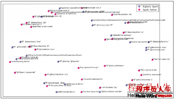
我们将通过画图来可视化结果。由于我们有6638个特点的7540个抽样,很难多维可视化,所以通过MDS算法来降维描绘 :
import matplotlib.pyplot as plt
import matplotlib as mpl
from sklearn.manifold import MDS
MDS() # # Bring down the MDS to two dimensions (components) as we will plot the clusters # mds = MDS(n_components=2, dissimilarity="precomputed", random_state=1)
pos = mds.fit_transform(dist) # shape (n_components, n_samples)
xs, ys = pos[:, 0], pos[:, 1]
In [67]: # # Set up colors per clusters using a dict # cluster_colors = {0: '#1b9e77', 1: '#d95f02', 2: '#7570b3', 3:'#e7298a', 4: '#66a61e', 5: '#9990b3', 6: '#e8888a'} # #set up cluster names using a dict # cluster_names = {0: 'Music, Pop', 1: 'USA Politics, Election', 2: 'BigData, Spark', 3: 'Spark, Python', 4: 'Thailand', 5: 'USA Politics, Election', 6: 'Music, Pop'}
In [115]: # # ipython magic to show the matplotlib plots inline # %matplotlib inline # # Create data frame which includes MDS results, cluster numbers and tweet texts to be displayed # df = pd.DataFrame(dict(x=xs, y=ys, label=clusters, txt=twtstxt_ls02_
utf8))
ix_start = 2000 ix_stop = 2050 df01 = df[ix_start:ix_stop]
print(df01[['label','txt']])
print(len(df01))
print() # Group by cluster groups = df.groupby('label')
groups01 = df01.groupby('label') # Set up the plot fig, ax = plt.subplots(figsize=(17, 10))
ax.margins(0.05) # # Build the plot object # for name, group in groups01:
ax.plot(group.x, group.y, marker='o', linestyle='', ms=12,
label=cluster_names[name], color=cluster_colors[name],
mec='none')
ax.set_aspect('auto')
ax.tick_params(\
axis= 'x', # settings for x-axis
which='both', #
bottom='off', #
top='off', #
labelbottom='off')
ax.tick_params(\
axis= 'y', # settings for y-axis
which='both', #
left='off', #
top='off', #
labelleft='off')
ax.legend(numpoints=1) # # # Add label in x,y position with tweet text # for i in range(ix_start, ix_stop):
ax.text(df01.ix[i]['x'], df01.ix[i]['y'], df01.ix[i]['txt'],
size=10)
plt.show() # Display the plot
label text 2000 2 b'RT @BigDataTechCon: ' 2001 3 b"@4Quant 's presentat" 2002 2 b'Cassandra Summit 201'
这是Cluster 2的图, 由蓝点表示Big Data 和 Spark; Cluster 3, 由红点表示Spark 和Python,和相干的 tweets 内容抽样 :
利用 Scikit-Learn 的处理结果,已探索到数据的1些好的见解,现在关注在Twitter数据集上履行 Spark MLlib。
预处理数据集
为了准备在数据集上运行聚类算法,现在聚焦特点提取和工程化。我们实例化Spark Context,读取 Twitter 数据集到1个 Spark dataframe. 然后,对tweet文本数据连续分词,利用哈希词频算法到 tokens, 并终究利用 Inverse Document Frequency 算法,重新缩放数据 。代码以下:
In [3]: import pandas as pd
csv_in = '/home/an/spark/spark⑴.5.0-bin-hadoop2.6/examples/AN_Spark/data/unq_tweetstxt.csv' pddf_in = pd.read_csv(csv_in, index_col=None, header=0, sep=';',encoding='utf⑻')
In [4]:
sqlContext = SQLContext(sc)
In [5]: spdf_02 = sqlContext.createDataFrame(pddf_in[['id', 'user_id', 'user_name', 'tweet_text']])
In [8]:
spdf_02.show()
In [7]:
spdf_02.take(3)
Out[7]:
[Row(id=638830426971181057, user_id=3276255125, user_name=u'True Equality', tweet_text=u'ernestsgantt: BeyHiveInFrance: 9_A_6:dreamintentions: elsahel12: simbata3: JDHM2015: almtorta18:dreamintentions:\u2026 http://t.co/VpD7FoqMr0'),
Row(id=638830426727911424, user_id=3276255125, user_name=u'True
Equality', tweet_text=u'ernestsgantt: BeyHiveInFrance:
PhuketDailyNews: dreamintentions: elsahel12: simbata3: JDHM2015:almtorta18: CiviPa\u2026 http://t.co/VpD7FoqMr0'),
Row(id=638830425402556417, user_id=3276255125, user_name=u'True
Equality', tweet_text=u'ernestsgantt: BeyHiveInFrance: 9_A_6:
ernestsgantt: elsahel12: simbata3: JDHM2015: almtorta18:
CiviPartnership: dr\u2026 http://t.co/EMDOn8chPK')]
In [9]: from pyspark.ml.feature import HashingTF, IDF, Tokenizer
In [10]: tokenizer = Tokenizer(inputCol="tweet_text",outputCol="tokens")
tokensData = tokenizer.transform(spdf_02)
In [11]:
tokensData.take(1)
Out[11]:
[Row(id=638830426971181057, user_id=3276255125, user_name=u'True Equality', tweet_text=u'ernestsgantt: BeyHiveInFrance:9_A_6: dreamintentions: elsahel12: simbata3: JDHM2015:almtorta18: dreamintentions:\u2026 http://t.co/VpD7FoqMr0',
tokens=[u'ernestsgantt:', u'beyhiveinfrance:', u'9_a_6:', u'dreamintentions:', u'elsahel12:', u'simbata3:', u'jdhm2015:',u'almtorta18:', u'dreamintentions:\u2026', u'http://t.co/vpd7foqmr0'])]
In [14]: hashingTF = HashingTF(inputCol="tokens", outputCol="rawFeatures",numFeatures=2000)
featuresData = hashingTF.transform(tokensData)
In [15]:
featuresData.take(1)
Out[15]:
[Row(id=638830426971181057, user_id=3276255125, user_name=u'True Equality', tweet_text=u'ernestsgantt: BeyHiveInFrance:9_A_6: dreamintentions: elsahel12: simbata3: JDHM2015:almtorta18: dreamintentions:\u2026 http://t.co/VpD7FoqMr0',
tokens=[u'ernestsgantt:', u'beyhiveinfrance:', u'9_a_6:', u'dreamintentions:', u'elsahel12:', u'simbata3:', u'jdhm2015:',u'almtorta18:', u'dreamintentions:\u2026', u'http://t.co/vpd7foqmr0'],
rawFeatures=SparseVector(2000, {74: 1.0, 97: 1.0, 100: 1.0, 160: 1.0,185: 1.0, 742: 1.0, 856: 1.0, 991: 1.0, 1383: 1.0, 1620: 1.0}))]
In [16]: idf = IDF(inputCol="rawFeatures", outputCol="features")
idfModel = idf.fit(featuresData)
rescaledData = idfModel.transform(featuresData) for features in rescaledData.select("features").take(3):
print(features)
In [17]:
rescaledData.take(2)
Out[17]:
[Row(id=638830426971181057, user_id=3276255125, user_name=u'True Equality', tweet_text=u'ernestsgantt: BeyHiveInFrance:9_A_6: dreamintentions: elsahel12: simbata3: JDHM2015:almtorta18: dreamintentions:\u2026 http://t.co/VpD7FoqMr0',
tokens=[u'ernestsgantt:', u'beyhiveinfrance:', u'9_a_6:', u'dreamintentions:', u'elsahel12:', u'simbata3:', u'jdhm2015:',u'almtorta18:', u'dreamintentions:\u2026', u'http://t.co/vpd7foqmr0'],
rawFeatures=SparseVector(2000, {74: 1.0, 97: 1.0, 100: 1.0, 160:1.0, 185: 1.0, 742: 1.0, 856: 1.0, 991: 1.0, 1383: 1.0, 1620: 1.0}),
features=SparseVector(2000, {74: 2.6762, 97: 1.8625, 100: 2.6384, 160:2.9985, 185: 2.7481, 742: 5.5269, 856: 4.1406, 991: 2.9518, 1383:4.694, 1620: 3.073})),
Row(id=638830426727911424, user_id=3276255125, user_name=u'True
Equality', tweet_text=u'ernestsgantt: BeyHiveInFrance:
PhuketDailyNews: dreamintentions: elsahel12: simbata3:
JDHM2015: almtorta18: CiviPa\u2026 http://t.co/VpD7FoqMr0',
tokens=[u'ernestsgantt:', u'beyhiveinfrance:', u'phuketdailynews:',u'dreamintentions:', u'elsahel12:', u'simbata3:', u'jdhm2015:',u'almtorta18:', u'civipa\u2026', u'http://t.co/vpd7foqmr0'],
rawFeatures=SparseVector(2000, {74: 1.0, 97: 1.0, 100: 1.0, 160:1.0, 185: 1.0, 460: 1.0, 987: 1.0, 991: 1.0, 1383: 1.0, 1620: 1.0}),
features=SparseVector(2000, {74: 2.6762, 97: 1.8625, 100: 2.6384,160: 2.9985, 185: 2.7481, 460: 6.4432, 987: 2.9959, 991: 2.9518, 1383:4.694, 1620: 3.073}))]
In [21]:
rs_pddf = rescaledData.toPandas()
In [22]:
rs_pddf.count()
Out[22]:
id 7540 user_id 7540 user_name 7540 tweet_text 7540 tokens 7540 rawFeatures 7540 features 7540 dtype: int64
In [27]:
feat_lst = rs_pddf.features.tolist()
In [28]:
feat_lst[:2]
Out[28]:
[SparseVector(2000, {74: 2.6762, 97: 1.8625, 100: 2.6384, 160: 2.9985,185: 2.7481, 742: 5.5269, 856: 4.1406, 991: 2.9518, 1383: 4.694, 1620: 3.073}),
SparseVector(2000, {74: 2.6762, 97: 1.8625, 100: 2.6384, 160: 2.9985,185: 2.7481, 460: 6.4432, 987: 2.9959, 991: 2.9518, 1383: 4.694, 1620:3.073})]
运行聚类算法
在Twitter数据集上运行 K-Means 算法, 作为非标签的tweets, 希望看到Apache Spark tweets 构成1个聚类。 遵从之前的步骤, 特点的 TF-IDF 稀疏向量转化为1个 RDD 将被输入到 Spark MLlib 程序。初始化 K-Means 模型为 5 聚类, 10 次迭代:
In [32]: from pyspark.mllib.clustering import KMeans, KMeansModel from numpy import array from math import sqrt
In [34]: in_Data = sc.parallelize(feat_lst)
In [35]:
in_Data.take(3)
Out[35]:
[SparseVector(2000, {74: 2.6762, 97: 1.8625, 100: 2.6384, 160: 2.9985,185: 2.7481, 742: 5.5269, 856: 4.1406, 991: 2.9518, 1383: 4.694, 1620:3.073}),
SparseVector(2000, {74: 2.6762, 97: 1.8625, 100: 2.6384, 160: 2.9985,185: 2.7481, 460: 6.4432, 987: 2.9959, 991: 2.9518, 1383: 4.694, 1620:3.073}),
SparseVector(2000, {20: 4.3534, 74: 2.6762, 97: 1.8625, 100: 5.2768,185: 2.7481, 856: 4.1406, 991: 2.9518, 1039: 3.073, 1620: 3.073, 1864:4.6377})]
In [37]:
in_Data.count()
Out[37]: 7540 In [38]: clusters = KMeans.train(in_Data, 5, maxIterations=10,
runs=10, initializationMode="random")
In [53]: def error(point): center = clusters.centers[clusters.predict(point)] return sqrt(sum([x**2 for x in (point - center)]))
WSSSE = in_Data.map(lambda point: error(point)).reduce(lambda x, y: x + y)
print("Within Set Sum of Squared Error = " + str(WSSSE))
评估模型和结果
聚类算法调优的1个方式是改变聚类的个数并验证输出. 检查这些聚类,感受1下目前的聚类结果:
In [43]:
cluster_membership = in_Data.map(lambda x:clusters.predict(x)) In [54]:
cluster_idx = cluster_membership.zipWithIndex() In [55]: type(cluster_idx) Out[55]:
pyspark.rdd.PipelinedRDD In [58]:
cluster_idx.take(20) Out[58]:
[(3, 0),
(3, 1),
(3, 2),
(3, 3),
(3, 4),
(3, 5),
(1, 6),
(3, 7),
(3, 8),
(3, 9),
(3, 10),
(3, 11),
(3, 12),
(3, 13),
(3, 14),
(1, 15),
(3, 16),
(3, 17),
(1, 18),
(1, 19)] In [59]:
cluster_df = cluster_idx.toDF() In [65]:
pddf_with_cluster = pd.concat([pddf_in, cluster_pddf],axis=1) In [76]:
pddf_with_cluster._1.unique() Out[76]: array([3, 1, 4, 0, 2]) In [79]:
pddf_with_cluster[pddf_with_cluster['_1'] == 0].head(10) Out[79]:
Unnamed: 0 id created_at user_id user_name tweet_text _1 _2 6227 3 642418116819988480 Fri Sep 11 19:23:09 +0000 2015 49693598 Ajinkya Kale RT @bigdata: Distributed Matrix Computations
i... 0 6227 6257 45 642391207205859328 Fri Sep 11 17:36:13 +0000 2015 937467860 Angela Bassa [Auto] I'm reading ""Distributed Matrix
Comput... 0 6257
6297 119 642348577147064320 Fri Sep 11 14:46:49 +0000
2015 18318677 Ben Lorica Distributed Matrix Computations in @
ApacheSpar... 0 6297
In [80]:
pddf_with_cluster[pddf_with_cluster['_1'] == 1].head(10)
Out[80]:
Unnamed: 0 id created_at user_id user_name tweet_text _1
_2
6 6 638830419090079746 Tue Sep 01 21:46:55 +0000 2015
2241040634 Massimo Carrisi Python:Python: Removing \xa0 from
string? - I ... 16
15 17 638830380578045953 Tue Sep 01 21:46:46 +0000 2015
57699376 Rafael Monnerat RT @ramalhoorg: Noite de autógrafos do
Fluent ... 115
18 41 638830280988426250 Tue Sep 01 21:46:22 +0000 2015
951081582 Jack Baldwin RT @cloudaus: We are 3/4 full! 2-day @
swcarpen... 1 18
19 42 638830276626399232 Tue Sep 01 21:46:21 +0000 2015
6525302 Masayoshi Nakamura PynamoDB #AWS #DynamoDB #Python
http://... 1 19
20 43 638830213288235008 Tue Sep 01 21:46:06 +0000 2015
3153874869 Baltimore Python Flexx: Python UI tookit based on web
technolog... 1 20
21 44 638830117645516800 Tue Sep 01 21:45:43 +0000 2015
48474625 Radio Free Denali Hmm, emerge --depclean wants to remove
somethi... 1 21
22 46 638829977014636544 Tue Sep 01 21:45:10 +0000 2015
154915461 Luciano Ramalho Noite de autógrafos do Fluent Python no
Garoa ... 122
23 47 638829882928070656 Tue Sep 01 21:44:47 +000