随机采样和随机模拟：吉布斯采样Gibbs Sampling实现文档分类

http://blog.csdn.net/pipisorry/article/details/51525308

吉布斯采样的实现问题

本文主要说明如何通过吉布斯采样进行文档分类（聚类），固然更复杂的实现可以看看吉布斯采样是如何采样LDA主题散布的[主题模型TopicModel：隐含狄利克雷散布LDA]。

关于吉布斯采样的介绍文章都停止在吉布斯采样的详细描写上，如随机采样和随机摹拟：吉布斯采样Gibbs Sampling(why)但并没有说明吉布斯采样到底如何实现的(how)？

也就是具体怎样实现从下面这个公式采样？

怎样在模型中处理连续参数问题？

怎样生成终究我们感兴趣的公式的期望值，而不是仅仅做T次随机游走？

下面介绍如作甚朴素贝叶斯Na ̈ıve Bayes[几率图模型：贝叶斯网络与朴素贝叶斯网络]构建1个吉布斯采样器，其中包括两大问题：如何利用共轭先验？如何通过等式14的条件中进行实际的几率采样？

皮皮blog

朴素贝叶斯模型的吉布斯采样器

问题

基于朴素贝叶斯框架，通过吉布斯采样对文档进行（无监督和有监督）分类。假定features是文档下的词，我们要预测的是doc-level的文档分类标签（sentiment label），值为0或1。

首先在无监督数据上进行朴素贝叶斯的采样，对监督数据的简化会在后面说明。

Following Pedersen [T. Pedersen. Knowledge lean word sense disambiguation. In AAAI/IAAI, page 814, 1997.,    T. Pedersen. Learning Probabilistic Models of Word Sense Disambiguation. PhD thesis, Southern Methodist University, 1998. http://arxiv.org/abs/0707.3972.], we’re going to describe the Gibbs sampler in a completely unsupervised setting where no labels at all are provided as training data.

模型表示

朴素贝叶斯模型对应的plate-diagram：

   

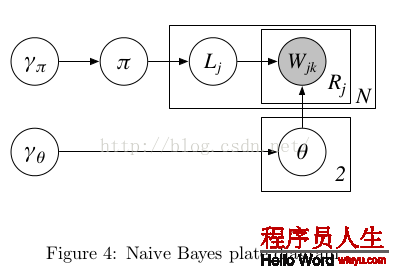
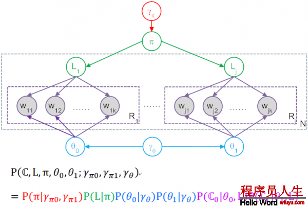
                                                                                                                                                                                         Figure4⑴

变量代表的意思以下表：

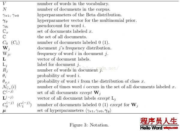
1.每个文档有1个Label(j)，是文档的class，同时θ0和θ1是和Lj对应的，如果Lj=1则对应的就是θ1

3.在这个model中，Gibbs Sampling所谓的P(Z)，就是产生图中这全部数据集的联合几率，也就是产生这N个文档整体联合几率，还要算上包括超参γ产生具体π和 θ的几率。所以最后得到了上图中表达式与对应色采。

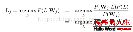
给定文档，我们要选择文档的label L使下面的几率越大：

文档生成进程

文档j的label生成

文档j的词袋生成描写

先验Priors

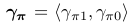
π来自哪里？

hyperparameters : parameters of a prior, which is itself used to pick parameters of the model.

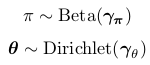
Our generative story is going to assume that before this whole process began, we also picked π randomly. Specifically we’ll assume that π is sampled from a Beta distribution with parameters γ π1 and γ π0 .

In Figure 4 we represent these two hyperparameters as a single two-dimensional vector γ π = γ π1 , γ π0 . When γ π1 = γ π0 = 1, Beta(γ π1 , γ π0 ) is just a uniform distribution, which means that any value for π is equally likely. For this reason we call Beta(1, 1) an “uninformed prior”.

θ 0 和 θ 1来自哪里？

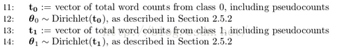
Let γ θ be a V -dimensional vector where the value of every dimension equals 1. If θ0 is sampled from Dirichlet(γθ ), every probability distribution over words will be equally likely. Similarly, we’ll assume θ 1 is sampled from Dirichlet(γ θ ).

Note: θ0为label为0的文档中词的几率散布；θ1为label为1的文档中词的几率散布。θ0and θ1are sampled separately. There’s no assumption that they are related to each other at all.

2.3 模型的状态空间和初始化

状态空间

朴素贝叶斯模型中状态空间的变量定义

• one scalar-valued variable π （文档j的label为1的几率）
• two vector-valued variables, θ 0 and θ 1
• binary label variables L, one for each of the N documents
We also have one vector variable W j for each of the N documents, but these are observed variables, i.e.their values are already known (and which is why W jk is shaded in Figure 4).

初始化

Pick a value π by sampling from the Beta(γ π1 , γ π0 ) distribution. sample出文档j的label为1的几率，也就知道了文档j的label的bernoulli几率散布(π, 1-π)。

Then, for each j, flip a coin with success probability π, and assign label L j(0)— that is, the label of document j at the 0 th iteration – based on the outcome of the coin flip. 通过上步得到的bernoulli散布sample出文档的label。

Similarly,you also need to initialize θ 0 and θ 1 by sampling from Dirichlet(γ θ ).

派生联合散布

for each iteration t = 1 . . . T of sampling, we update every variable defining the state space by sampling from its conditional distribution given the other variables, as described in equation (14).

处理进程：

• We will define the joint distribution of all the variables, corresponding to the numerator in (14).
• We simplify our expression for the joint distribution.
• We use our final expression of the joint distribution to define how to sample from the conditional distribution in (14).
• We give the final form of the sampler as pseudocode.

联合散布的表示和简化

模型对全部文档集的联合散布为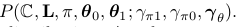

Note： 分号右侧是联合散布的参数，也就是说分号左侧的变量是被右侧的超参数条件住的。

联合散布可分解为（通过图模型）：

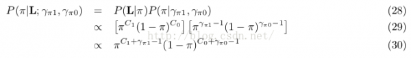
因子1：

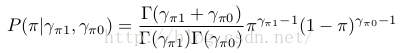
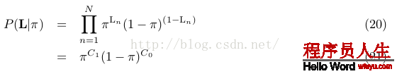
也即Figure4⑴红色部份：这个是从beta散布sample出1个伯努利散布，伯努利散布只有1个参数就是π，不要normalization项（要求的是全部联合几率，所以在这里纠结normalization是没有用的），得到：

因子2：

也即Figure4⑴绿色部份：这里L是1全部向量，其中值为0的有C0个，值为1的有C1个，屡次伯努利散布就是2项散布啦，因此：

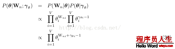
因子3：

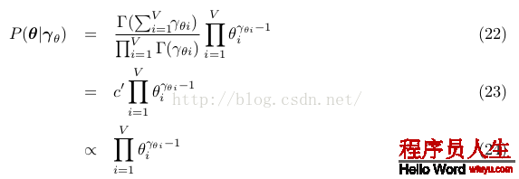
词的散布几率，也即Figure4⑴蓝色部份：对0类和1类的两个θ都采样自参数为γθ的狄利克雷散布，注意所有这些都是向量，有V维，每维度对应1个Word。根据狄利克雷的PDF得到以下表达式，其实这个表达式有两个，分别为θ0和θ1用相同的式子采样：

因子4：

P (C 0 |θ 0 , L) and P (C 1 |θ 1 , L): the probabilities of generating the contents of the bags of words in each of the two document classes.

也即Figure4⑴紫色部份：首先要求对单唯一个文档n，产生所有word也就是Wn的几率。假定对某个文档，θ=(0.2,0.5,0.3)，意思就是word1产生几率0.2，word2产生几率0.5，假设这个文档里word1有2个，word2有3个，word3有2个，则这个文档的产生几率就是(0.2*0.2)*(0.5*0.5*0.5)*(0.3*0.3)。所以依照这个道理，1个文档全部联合几率以下：

let θ = θ L n:

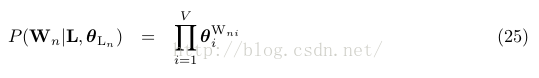
Wni: W n中词i的频数。

文档间相互独立，同1个class中的文档合并，上面这个几率是针对单个文档而言的，把所有文档的这些几率乘起来，就得到了Figure4⑴紫色部份：

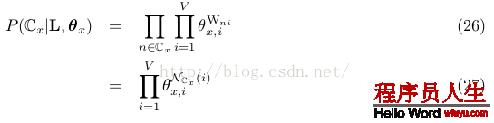
Note: 其中x的取值可以是0或1，所以Cx可以是C0或C1，当x=0时，n∈Cx的意思就是对所有class 0中的文档，然后对这些文档中每个word i，word i在该文档中出现Wni次，求θ0,i的Wni次方，所有这些乘起来就是紫色部份。后式27是规约后得到的结果，NCx (i) ：word i在 documents with class label x中的计数，如NC0(i)的意思就是word i出现在calss为0的所有文档中的总数，同理对NC1(i)。

联合散布的表示和先验选择的缘由

使用式19和21：

使用式24和25：

如果使用所有文档的词（也就是使用式24和27）

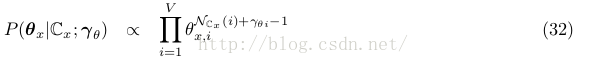
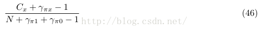
可知后验散布式30是1个unnormalized Beta distribution, with parameters C 1 + γ π1 and C 0 + γ π0 ,且式32是1个unnormalized Dirichlet distribution, with parameter vector N C x (i) + γ θi for 1 ≤ i ≤ V .

也就是说先验和后验散布是1种情势，这样Beta distribution是binomial (and Bernoulli)散布的共轭先验，Dirichlet散布是多项式multinomial散布的共轭先验。
而超参数就如视察到的证据，是1个伪计数pseudocounts。

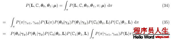
让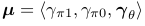，全部文档集的联合散布表示为：

将隐含变量π积出

why: 为了方便，可以对隐含变量π进行积分，最后到达消去这个变量的目的。我们可以通过积分掉π来减少模型有效的参数个数。This has the effect of taking all possible values of π into account in our sampler, without representing it as a variable explicitly and having to sample it at every iteration. Intuitively, “integrating out” a variable is an application of precisely the same principle as computing the marginal probability for a discrete distribution.As a result, c is “there” conceptually, in terms of our understanding of the model, but we don’t need to deal with manipulating it explicitly as a parameter.

Note: 积分掉的意思就是

因而联合散布的边沿散布为：

只斟酌积分项：

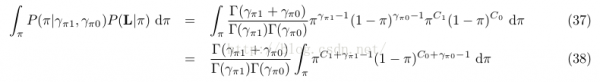
而38式后面的积分项是1个参数为C 1 + γ π1 and C 0 + γ π0的beta散布，且Beta(C 1 + γ π1 , C 0 + γ π0 )的积分为

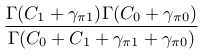
让N = C 0 + C 1

则38式表示为：

全部文档集的联合散布表示（3因子式）为：

其中，N = C 0 + C 1

构建吉布斯采样器Gibbs Sampler

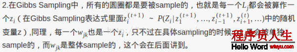
吉布斯采样就是通过条件几率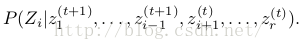给Zi1个新值

如要计算，需要计算条件散布

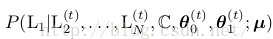
Note: There’s no superscript on the bags of words C because they’re fully observed and don’t change from iteration to iteration.

要计算θ 0，需要计算条件散布

直觉上，在每一个迭代t开始前，我们有以下当前信息：

每篇文档的词计数，标签为0的文档计数，标签为1的文档计数，每篇文档确当前label，θ0 和 θ1确当前值等等。

采样准则

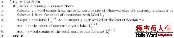
采样label：When we want to sample the new label for document j, we temporarily remove all information (i.e. word counts and label information) about this document from that collection of information. Then we look at the conditional probability that L j = 0 given all the remaining information, and the conditional probability that L j = 1 given the same information, and we sample the new label L j (t+1) by choosing randomly according to the relative weight of those two conditional probabilities.

采样θ：Sampling to get the new values operates according to the same principal.

2.5.1 文档标签的采样

定义条件几率

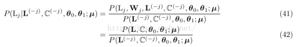
L (−j) are all the document labels except L j , and C (−j) is the set of all documents except W j .

份子是全联合几率散布，分母是除去Wj信息的相同的表达式，所以我们需要斟酌的只是式40的3个因子。

其实我们要做的只是斟酌除去Wj后，改变了甚么。

因子1

由于因子1仅依赖于超参数，份子分母1样，不予斟酌，故只斟酌式40中的因子2和因子3。

因子2

式42因子2分母的计算与上1次迭代Lj是多少有关。

不过语料大小总是从N变成了N⑴，且其中1个文档种别的计数减少1。如Lj=0，则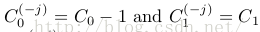，Cx只有1个有变化，这样

let x be the class for which C x(−j)= C x − 1，式42的因子2重写为：

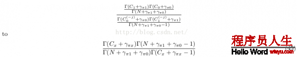
又Γ(a + 1) = aΓ(a) for all a

这样式42的因子2简化为：

因子3

同因子2，总有某个class对应的项没变，也就是式42的因子3中θ 0 or θ 1有1项在份子和分母中是1样的。

合并

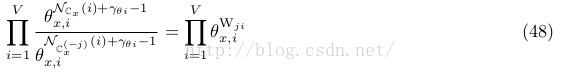
for x ∈ {0, 1}，终究合并得到采样文档label的的条件散布为

从式49看文档的label是如何选择出来的：

式49因子1：L j = x considering only the distribution of the other labels

式49因子2：is like a word distribution “fitting room.”, an indication of how well the words in W j “fit” with each of the two distributions.

前半部份其实只有Cx是变量，所以如果C0大，则P(L(t+1)j=0)的几率就会大1点，所以下1次Lj的值就会偏向于C0，反之就会偏向于C1。而后半部份，是在判断当前θ参数的情况下，全部文档的likelihood更偏向于C0还是C1。

式42的条件散布采样进程以下

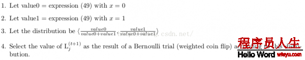
Note: 步骤3是对两个label的几率散布进行归1化。

对监督数据

Using labeled documents just don’t sample L j for those documents! Always keep L j equal to the observed label.

The documents will effectively serve as “ground truth” evidence for the distributions that created them. Since we never sample for their labels, they will always contribute to the counts in (49) and (51) and will never be subtracted out.

2.5.2 θ的采样

由于θ 0 and θ 1的散布估计是独立的，这里我们先消去θ下标。

明显

since we used conjugate priors, this posterior, like the prior, works out to be a Dirichlet distribution. We actually derived the full expression , but we don’t need the full expression here. All we need to do to sample a new distribution is to make another draw from a Dirichlet distribution, but this time with parameters N C x (i) + γ θi for each i in V .

define the V dimensional vector t such that each 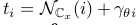（这里i下标代表V维向量t的第i个元素）:

new θ的采样公式

从Dirichlet散布采样的实现

sample a random vector a = <a 1 , . . . , a V> from the V -dimensional Dirichlet distribution with parameters <α 1 , . . . , α V>

最快的实现是draw V independent samples y 1 , . . . , y V from gamma distributions, each with density

然后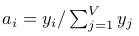（也就是正则化gamma散布的采样）

[http://en.wikipedia.org/wiki/Dirichlet distribution]

全部朴素贝叶斯模型的吉布斯采样框架

模型初始化

=<1, 1>   uninformed prior: uniform distribution

=<1, ..., 1>   Let γθ be a V-dimensional vector where the value of every dimension equals 1.   uninformed prior

Pick a value π by sampling from the Beta(γ π1 , γ π0 ) distribution. sample出文档j的label为1的几率，也就知道了文档j的label的bernoulli几率散布(π, 1-π)。

Then, for each j, flip a coin with success probability π, and assign label L j(0)— that is, the label of document j at the 0 th iteration – based on the outcome of the coin flip. 通过上步得到的bernoulli散布sample出文档的label。

Similarly,you also need to initialize θ 0 and θ 1 by sampling from Dirichlet(γθ ).

模型迭代

2.5.1 文档j标签label的采样公式

2.5.2 θ采样中的（这里i下标代表V维向量t的第i个元素）

Note: lz: 如果要并行计算，特别注意的变量主要只有3个：，，

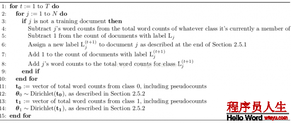
算 法中第3步好像写错了，应当去掉not?

Note:  as soon as a new label for L j is assigned, this changes the counts that will affect the labeling of the subsequent documents. This is, in fact, the whole principle behind a Gibbs sampler!

从吉布斯采样中产生值

吉布斯采样算法的初始化和采样迭代都会产生每一个变量的值（for iterations t = 1, 2, . . . , T），In theory, the approximated value for any variable Z i can simply be obtained by calculating:

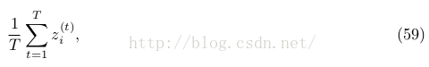
正如我们所知，吉布斯采样迭代进入收敛阶段才是稳定散布，所以1般式59加和不是从1开始，而是B + 1 through T，要抛弃t < B的采样结果。

In this context, Jordan Boyd-Graber (personal communication) also recommends looking at Neal’s [15] discussion of likelihood as a metric of convergence.

皮皮blog

PS

1 2.6 Optional: A Note on Integrating out Continuous Parameters

In Section 3 we discuss how to actually obtain values from a Gibbs sampler, as opposed to merely watching it walk around the state space. (Which might be entertaining, but wasn’t really the point.) Our discussion includes convergence and burn-in, auto-correlation and lag, and other practical issues.

In Section 4 we conclude with pointers to other things you might find it useful to read, as well as an invitation to tell us how we could make this document more accurate or more useful.

同步图计算并行化处理

lz的不1定正确。。。

将文档数据分成M份，散布在M个worker节点中。

超步1：所有节点运行朴素贝叶斯吉布斯采样算法的模型初始化部份，得到，，的初始值

超步2+：

超步开始前，主节点通过其它节点发来的改变的增量信息计算的新值，并分发给worker所有节点。（全局模型）

每一个节点保存有自己的信息，收到其它节点发来的改变的增量信息，主节点发来的信息

重新运行重新朴素贝叶斯吉布斯采样算法的模型的迭代部份，计算新值（局部模型）

全部节点的数据迭代完成后计算改变的增量信息，并在超步结束后发给主节点。

burn-in阶段抛弃所有节点采样结果；收敛阶段将所有节点得到的采样结果：所有文档的标签值记录下来。

全部进程进行屡次迭代，最后文档的标签值就是所有迭代得到的向量[标签值]的均值偏向的标签值。

还有1种同步图并行计算多是这样?

类似Spark MLlib LDA 基于GraphX实现原理，以文档到词作为边，以词频作为边数据，把语料库构造成图，把对语料库中每篇文档的每一个词操作转化为在图中每条边上的操作，而对边RDD处理是GraphX中最多见的的处理方法。 

[Spark MLlib LDA 基于GraphX实现原理及源码分析]

基于GraphX实现的Gibbs Sampling LDA，定义文档与词的2部图，顶点属性为文档或词所对应的topic向量计数，边属性为Gibbs Sampler采样生成的新1轮topic。每轮迭代采样生成topic，用mapReduceTriplets函数为文档或词累加对应topic计数。这好像是Pregel的处理方式？Pregel实现过LDA。

[基于GraphX实现的Gibbs Sampling LDA]

[Collapsed Gibbs Sampling for LDA]

[LDA中Gibbs采样算法和并行化]

from: http://blog.csdn.net/pipisorry/article/details/51525308

ref:  Philip Resnik : GIBBS SAMPLING FOR THE UNINITIATED*

Reading Note : Gibbs Sampling for the Uninitiated